Predicting ‘Wait time’ categories for On-Demand Food Delivery Service Using Smartphone Dataset
Ashok K Yannam
Experiment and Data Collection
This experiment has been carried out by simulating myself as an UberEats/DoorDash driver for three different trips and restaurants. Each trip performed five activities (WALKING, DRIVING, SITTING, STANDING, LAYING) with a smartphone (iPhone X). Using its embedded sensors GPS, IMI, etc., captured the data during entire duration of each trip at a constant rate of 1 Hz. For each record it is provided:
- CLLocation: latitude, longitude, altitude, speed, course, verticalAccuracy, horizontalAccuracy, floor
- CLHeading: heading.x, heading.y, heading.z, trueHeading, magneticHeading, headingAccuracy
- Core ML Model output (supported type int, double, string, dictionary)
- CMMotionActivity: Activity, activity.startDate, activity.confidence
- CMAltimeter: relativeAltitude, pressure
- WIFI and network carrier IP addresses
- Device orientation
The datasets are preprocessed and manually labeled to create dataset to use for training and test dataset with below data points
- CLLocation: latitude, longitude, speed of the driver
- CMMotionActivity: Activity, activity.startDate, activity.confidence of the driver
- Timestamps, Sample numbers, latitude & longtitude for restaurant and destination
Below are the frameworks used
- Pandas Documentation: http://pandas.pydata.org/
- Scikit Learn Documentation: http://scikit-learn.org/stable/documentation.html
- Seaborn Documentation: http://seaborn.pydata.org/
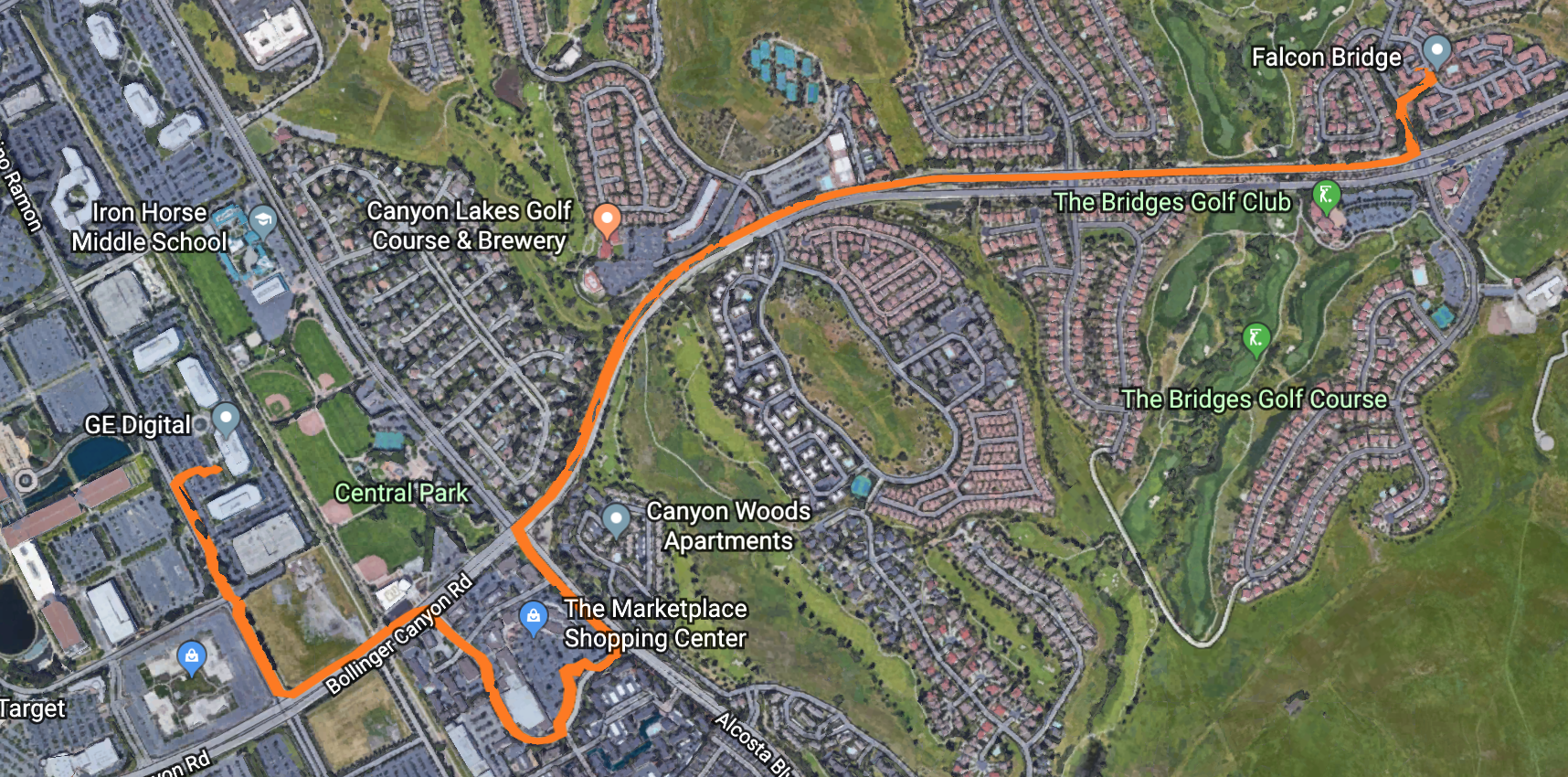
Trip 1
- Restaurant: Starbucks, Market place, San Ramon CA
- Destination: GE Digital, San Ramon CA
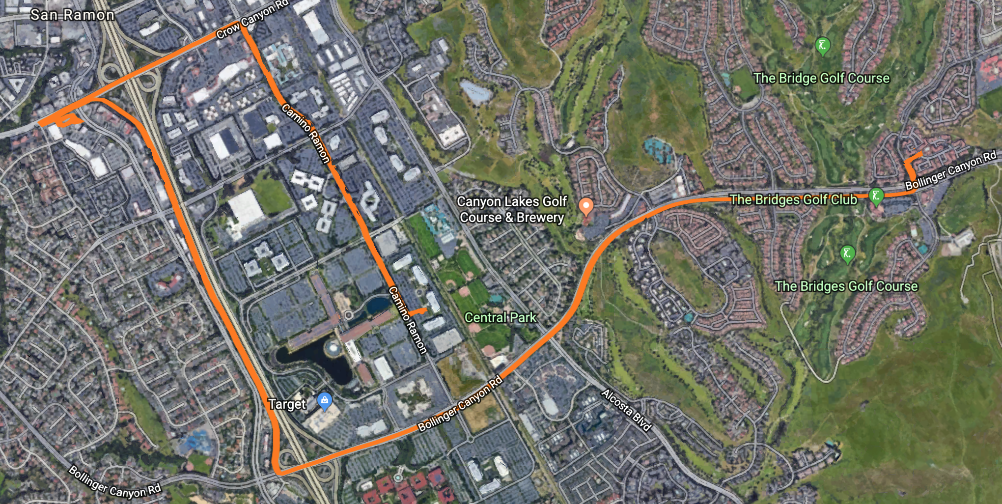
Trip 2
- Restaurant: Chipotle, San Ramon CA
- Destination: Falcon Bridge, San Ramon CA
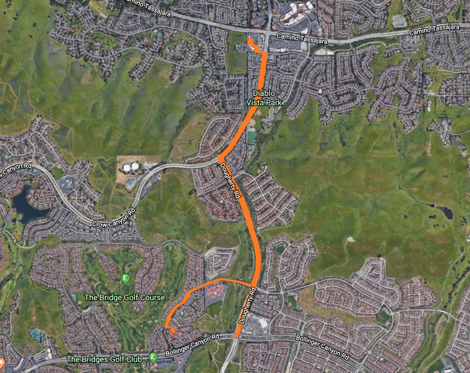
Trip 3
- Restaurant: Similan Thai, Danville CA
- Destination: Falcon Bridge, San Ramon CA
Import necessary libraries
In [1]:
import numpy as np
import pandas as pd
import matplotlib.pyplot as plt
%matplotlib inline
Data and Feature Engineering
In [2]:
df = pd.read_csv('processedDataset/onDemandFoodDelivery_AllTrips.csv')
In [3]:
df.head()
Out[3]:
In [4]:
df.info()
In [5]:
df['label'].value_counts()
Out[5]:
In [6]:
from math import radians, cos, sin, asin, sqrt

def haversine(lat1,lon1,lat2,lon2):
    """
    Calculate the great circle distance between two points
    on the earth (specified in decimal degrees)

    All args must be of equal length.

    """
    lon1, lat1, lon2, lat2 = map(np.radians, [lon1, lat1, lon2, lat2])

    dlon = lon2 - lon1
    dlat = lat2 - lat1

    a = np.sin(dlat/2.0)**2 + np.cos(lat1) * np.cos(lat2) * np.sin(dlon/2.0)**2

    c = 2 * np.arcsin(np.sqrt(a))
    km = 6371 * c # Radius of earth in kilometers. Use 3956 for mi
    meters = km
    return meters
In [7]:
X = df.locationSpeed
Y = df.activity
rlat = df['restLatitude']
rlong = df['restLongitude']
driverlat = df['locationLatitude']
driverlong = df['locationLongitude']
dlat = df['destLatitude']
dlong = df['destLongitude']
Z = haversine(rlat, rlong, driverlat, driverlong)
W = haversine(dlat, dlong, driverlat, driverlong)
In [10]:
plt.plot(X, label="Speed")
plt.plot(Y, label="Activity")
plt.plot(Z, label="Rstaurt Distance")
plt.plot(W, label="Dest Distance")

# Add legend
plt.legend(loc='upper left', fontsize=18)
# Add title and x, y labels
plt.title("Line Plot Sensor Data", fontsize=18, fontweight='bold')
plt.xlabel("Time", fontsize=18, fontweight='bold')
plt.ylabel("Sensor Values", fontsize=18, fontweight='bold')
plt.rcParams["figure.figsize"] = [16*2,9*2]
plt.show()

In [11]:
df.label.unique()
Out[11]:
In [12]:
import seaborn as sns
In [13]:
grid = sns.pairplot(df, hue='label', vars=['locationSpeed', 'activity', 'restDistance', 'destDistance'])
grid.fig.suptitle('OnDemand Food Delivery Time Series Data');

Classification with the features to predict target labels
1-hot encoding of features
In [14]:
features = df.drop('label', axis=1)
In [15]:
X = pd.get_dummies(features)
In [16]:
X.head()
Out[16]:
Label encoding
In [17]:
df['label'].value_counts()
Out[17]:
In [18]:
from sklearn.preprocessing import LabelEncoder
In [19]:
le = LabelEncoder()
y = le.fit_transform(df['label'])
le.classes_
Out[19]:
Train test split
In [20]:
from sklearn.model_selection import train_test_split
X_train, X_test, y_train, y_test = train_test_split(
    X, y, test_size=0.3, random_state=0)
Fit a Logistic Regression model
In [21]:
from sklearn.linear_model import LogisticRegression

model = LogisticRegression()
model.fit(X_train, y_train)
Out[21]:
In [22]:
y_pred = model.predict(X_test)
In [23]:
model.score(X_train, y_train)
Out[23]:
In [24]:
model.score(X_test, y_test)
Out[24]:
In [25]:
from sklearn.metrics import confusion_matrix, classification_report
In [26]:
confusion_matrix(y_test, y_pred)
Out[26]:
Looking at the scores of Logistic Regression, we can conclude this model is terrible on this time series data
Fit a Decision Tree model
In [27]:
from sklearn.tree import DecisionTreeClassifier
model = DecisionTreeClassifier(max_depth=2, random_state=33)
model.fit(X_train, y_train)
Out[27]:
In [28]:
y_pred = model.predict(X_test)
In [29]:
model.score(X_train, y_train)
Out[29]:
In [30]:
model.score(X_test, y_test)
Out[30]:
In [31]:
df['label'].value_counts()/len(df['label'])
Out[31]:
In [32]:
confusion_matrix(y_test, y_pred)
Out[32]:
In [33]:
model = DecisionTreeClassifier(max_depth=5, random_state=42)
model.fit(X_train, y_train)
model.score(X_test, y_test)
Out[33]:
In [34]:
model = DecisionTreeClassifier(max_depth=5, min_samples_leaf=5)
model.fit(X_train, y_train)
model.score(X_test, y_test)
Out[34]:
In [35]:
depths = range(1, 20)
scores_test = []
scores_train = []
for d in depths:
    model = DecisionTreeClassifier(max_depth=d)
    model.fit(X_train, y_train)
    s_train = model.score(X_train, y_train)
    s_test = model.score(X_test, y_test)
    scores_train.append(s_train)
    scores_test.append(s_test)

plt.plot(scores_train, label="TrainScore")
plt.plot(scores_test, label="TestScore")
plt.legend(loc='upper left', fontsize=18)
plt.ylabel('Scores', fontsize=18, fontweight='bold')
plt.xlabel('Max Depth', fontsize=18, fontweight='bold')
Out[35]:
